If you need an estimated pump flow reading but don’t want to install a separate flowmeter, the flow estimation (flowmeter function) in the Altivar Solar ATV320 can help. It uses the pump’s performance curve plus the drive’s actual load to estimate flow, then makes that value available for monitoring and other drive functions.
This post walks through the full configuration process: preconfiguration, picking five calibration points, measuring flow at each point (two ways), entering values into the drive, and checking results. You’ll also see what accuracy to expect so you can decide if sensorless flow estimation fits your application.
How Altivar ATV320 flow estimation works (and what accuracy to expect)
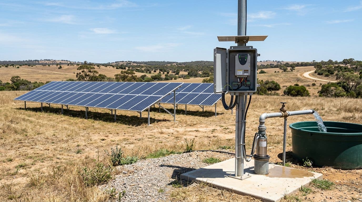 Solar pumping setup concept (drive plus pump and PV supply).
The flow estimation function provides an estimated flow value without a physical flowmeter. Instead of measuring flow directly, the drive estimates it from two key inputs:
- The pump manufacturer’s PQ (power/flow) performance curve, which relates pump behavior to flow output.
- The drive’s actual load, which reflects what the motor and pump are doing in real time.
To make this work, you store five operating points from the pump curve in the drive parameters (five power points and five flow points). Once calibrated, the drive uses those reference points to estimate flow across the operating range.
It’s important to set expectations up front. Even with good calibration and a low geometric height (with favorable installation conditions), the sensorless estimated flow function is still typically around plus or minus 20% accuracy, assuming a stable water level in the well or tank. In other words, it’s an estimate you can trend and use for basic control logic, not a replacement for a custody-grade measurement.
If you want the manufacturer’s documentation handy while you work, keep the Altivar Solar ATV320 user manual (PKR47019) nearby. It’s the best reference for parameter names and menu paths on your exact firmware and terminal.
Preconfiguration: set the drive up for stable testing and calibration
 Configuring a drive from the local graphic terminal.
Because this process depends on consistent pump behavior, start by creating stable test conditions. The guidance is to run these tests in optimum sunlight if you’re on PV, or perform them on the AC network (mains) if that’s available to you during commissioning.
From the drive menus, the preconfiguration sequence is:
- Go to the Configuration menu.
- Choose Full.
- Enter the Sun menu.
- Find Volume counter, then set Volume source to Flow estimation.
Next, the video calls out deactivating the PV supply algorithm (to avoid instability during the calibration activity). The goal here is consistent operation while you capture your five points.
There’s also a setting called Low voltage assign that affects behavior under supply variation:
- In sunny conditions, set Low voltage assign = No so the drive stays stable and can run at full speed during testing.
- When the drive is connected to the network (AC mains), set Low voltage assign = No.
- When running on solar panels in cloudy conditions, set Low voltage assign = Yes (so the drive can respond appropriately to low PV voltage).
- For the calibration tests themselves, keep Low voltage assign = No.
Once your flow estimation source is set and the supply behavior is stable, you’re ready to choose reference points and start collecting power and flow values.
For broader background on Schneider’s drive family (and where solar pumping fits in), see Schneider Altivar Series applications in renewable energy.
Pick the five reference points (low speed to high speed)
Flow estimation setup requires five reference points. Practically, that means you need five distinct operating speeds where you can record:
- Power value (PCP) at that speed
- Flow value (PCQ) at that speed
In the video example, low speed is 15 Hz because there’s no flow under 15 Hz. The high speed is 50 Hz.
To space five points evenly between low and high speed, use this approach:
- Subtract the low speed from the high speed.
- Divide the result by 4 (because five points create four intervals).
In the example:
- Low speed: 15 Hz
- High speed: 50 Hz
- Step size: (50 − 15) / 4 = 8.75 Hz, rounded to about 9 Hz
That gives these five reference points:
- 15 Hz
- 24 Hz
- 33 Hz
- 41 Hz
- 50 Hz
This spacing matters because it spreads your calibration across the operating range. If you only calibrate near one end, the estimate can drift when you run far from those points.
Add mechanical power (%) to the terminal display
Before recording values, update what the graphic display terminal shows so you can easily capture power at each test speed.
Go to the Interface menu, then Monitoring config. In the parameter selection (the video references “Pam bar”), select Motor mech power in percentage so power data appears in the right corner of the graphic display terminal. Unselect other parameters you don’t need for this task so the screen stays readable while you’re testing.
Record the power value (PCP) at each reference speed
At each reference frequency, run the drive and read the percentage of the maximum power shown by the drive (the video refers to this as “OPR”). Then calculate the power value PCP using the formula provided for the function.
Because the formula itself isn’t shown clearly here, follow the exact calculation method in Schneider’s documentation for your configuration. The official resources that match this procedure include the Schneider Electric FAQ page for this configuration video and the user manual referenced earlier.
Repeat the same “set speed, read power percent, compute PCP” process at:
- 15 Hz
- 24 Hz
- 33 Hz
- 41 Hz
- 50 Hz
Once you have five PCP values, you can move on to capturing the five flow values (PCQ).
Measure flow at each point: portable flowmeter or water meter method
You need a flow value at each reference point to complete calibration. The video offers two ways, depending on what instruments you have on site.
Method 1: Calibrate with a portable flowmeter (five points)
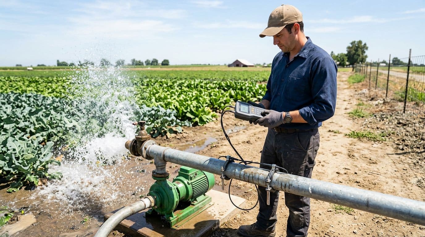 Measuring pump discharge flow with a portable flowmeter.
This is the most direct approach because you measure flow while the pump runs at each set frequency.
For each reference speed:
- Start the motor.
- Go to Simply start and set the High-speed (HSP) value to the reference frequency (15, 24, 33, 41, 50 Hz).
- Read the flow value on the portable flowmeter.
- Record that flow as the PCQ value for that point.
- At the same time, capture the power reading you need for PCP if you haven’t already.
Repeat until you have five flow values that correspond exactly to your five speeds.
A simple way to avoid mix-ups is to record power and flow together at each frequency, then move to the next frequency only after both values are written down.
Method 2: Use a water meter, or time a 10 L bucket fill
 Timing how long it takes to fill a known container to calculate flow.
- Water meter approach: Read the meter’s flow or totalized value over a known time window while the pump runs at a steady reference speed.
- Bucket timing approach: Fill a known volume container (the example uses a 10 L bucket or tank) and measure the fill time.
Then calculate flow using the standard relationship:
- Flow = Volume / Time
Just keep your units consistent. For example, liters per second can be converted to liters per minute by multiplying by 60. If you work in gallons, stay in gallons and seconds or minutes.
The key is consistency. Use the same container, repeat the timing if needed, and make sure the pump holds steady at each reference frequency long enough to get a reliable duration. After you compute the flow for a point, that value becomes your PCQ value for that speed.
Enter Flow 1 to Flow 5 and Power 1 to Power 5 in the drive (then verify)
Once you’ve collected five power values and five flow values, open the Flow estimation menu on the drive and enter your results:
- Fill Flow 1 through Flow 5
- Fill Power 1 through Power 5
To keep everything organized, map each frequency to the corresponding parameter pair. This table shows the structure (you’ll enter your measured numbers):
| Reference point | Frequency (Hz) | Drive flow parameter | Drive power parameter |
|---|---|---|---|
| 1 | 15 | Flow 1 (PCQ1) | Power 1 (PCP1) |
| 2 | 24 | Flow 2 (PCQ2) | Power 2 (PCP2) |
| 3 | 33 | Flow 3 (PCQ3) | Power 3 (PCP3) |
| 4 | 41 | Flow 4 (PCQ4) | Power 4 (PCP4) |
| 5 | 50 | Flow 5 (PCQ5) | Power 5 (PCP5) |
After you enter everything, check Estimated pump flow on the drive and compare it to your actual measurement (portable flowmeter reading, water meter reading, or your bucket calculation). In the video example, the estimated pump flow and the flowmeter reading match after entry and verification.
Finally:
- Stop the motor.
- Return the drive to your initial solar configuration (undo temporary test settings that you changed to stabilize calibration).
If you want a second reference for the same procedure in a written, step-based format, Schneider also maintains a related guide at Schneider Electric Community: flowmeter function on Altivar Solar ATV320.
Practical notes: when flow estimation is helpful (and when it isn’t)
Flow estimation is most useful when you need a reasonable trend without adding hardware. For example, it can support monitoring, basic control decisions, and features that require a flow value to be present.
Still, keep these real-world limits in mind:
- Accuracy is limited: about plus or minus 20% is a realistic expectation, even with good setup and stable water level.
- Changing conditions can shift results: water level changes in a well or tank, piping changes, or pump wear can all affect how closely the estimate matches reality.
- Calibration quality matters: the five points should be measured carefully, at stable speeds, and across the range you actually plan to run.
Schneider also notes in other drive families that estimated flow is not as precise as measured flow, especially when you use it to calculate totals over time. For background on that limitation, see Schneider guidance on flow estimation versus measured flow.
Conclusion
Configuring the flow estimation function on an Altivar Solar ATV320 comes down to stable test conditions, five well-spaced reference speeds, and careful power and flow measurements at each point. After you enter Flow 1 to Flow 5 and Power 1 to Power 5, the drive can estimate pump flow without installing a dedicated flowmeter. If you need higher accuracy than the estimate can provide, the same process also helps you decide where a physical flow sensor is worth the effort.